Embedding Twilight Imperium Maps in 3D space

• How to embed a graph in $n$-dimensional Euclidian Space
• Embedding a grid
• Planarising a Twilight Imperium Map
• How new wormholes change the geometry
• Actual Applications
• Implementation notes

Twilight Imperium (TI) is a board game about interstellar combat. All you need to know for the purposes of this post is that it is played on a hexagonal grid and that it features multiple kinds of wormholes. Two tiles count as adjacent if either they are touching or if they are wormholes of the same kind.

The wormholes mean that the game board doesn’t sit naturally in 2D Euclidian space. During the game, however, it is very easy for an amateur like me to loose track of that fact. If tiles are physically further away from me on the table, I am irrationally inclined to treat them as far away in terms of movement points.

I thought it would be useful to embed the game board in a higher dimensional space to get a feel for how everything is actually connected. This led me to learn about some cool maths.

How to embed a graph in $n$-dimensional Euclidian Space

There are many ways to do this, I went with Multidimensional scaling (MDS), as described in a paper¹ by Schwartz et al., because the key idea is very intuitive: Figure out how far apart your graph nodes should be and wiggle them about until it works. More formally,

1. Calculate all pairwise distances $g_{ij}$ in the graph between vertices $v_i$ and $v_j$.
2. For each vertex $v_i$, pick a random point $\mathbf {p}_i$ in $n$-dimensional space. Let’s call the collection of all these points $P$, and let’s define the Euclidian distance $d_{ij} = \left\lVert \mathbf {p}_i - \mathbf {p}_j \right\rVert$.
3. Define the loss function² $$\mathcal L = \sqrt{ \sum_{i, j} \left( g_{ij} - d_{ij} \right)^2 }.$$
4. Use your favourite optimizer³ to find the optimal positions $\hat P$: $$\hat P = \argmin_P \mathcal L$$

Schwartz et al. actually use a different loss function

$$\mathcal L_{ \text{local} } = \frac 1 {c} \sum_{i, j} \frac { \left( g_{ij} - d_{ij} \right)^2 } { d_{ij} }$$

where

$$c = \sum_{i, j} d_{ij}$$

is used for normalization. I have found that $\mathcal L_{ \text{local} }$ doesn’t preserve global structure as well as $\mathcal L$.

Embedding a grid

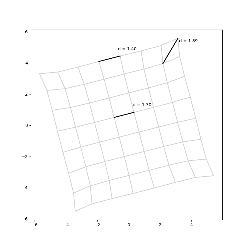
We want to embed a hexagonal grid with wormholes, but as a proof of concept I tried embedding a simple 8x8 grid, with the Manhattan distance $g_{i,j} = \Delta x + \Delta y$. This is the distance function you would use for a game board where pieces can only move to adjacent (square) cells. Here you can see the algorithm at work:

It recovers a grid! It succeeds most of the time, although sometimes it gets into weird local maxima⁴:

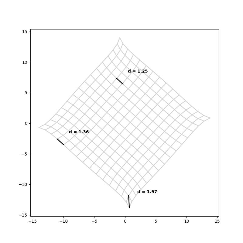
Interestingly, even though the graph distances between adjacent grid notes are 1, their distances in the embedding are around 1.3, which seems to be a comprimise between Manhattan and Euclidian distances. The edges and particularly the corners are fleeing the centre a bit.

The warping gets stronger and the graph shrinks together more on larger grids.

The loss function affects the amount of warping. Let’s look at the generalised loss function of order k:

$$\mathcal L_k = \sqrt[k]{ \sum_{i, j} \left| g_{ij} - d_{ij} \right|^k }.$$

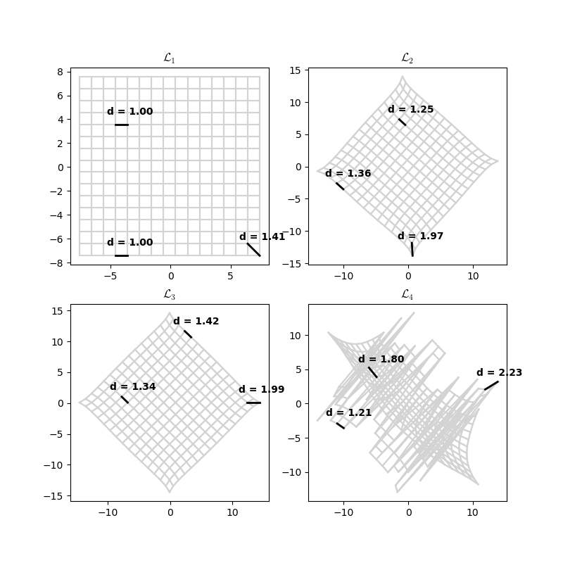
$\mathcal L_1$ recovers the full grid, which makes sense because it’s just the Manhattan distance. $\mathcal L_4$ is not happy.

Planarising a Twilight Imperium Map

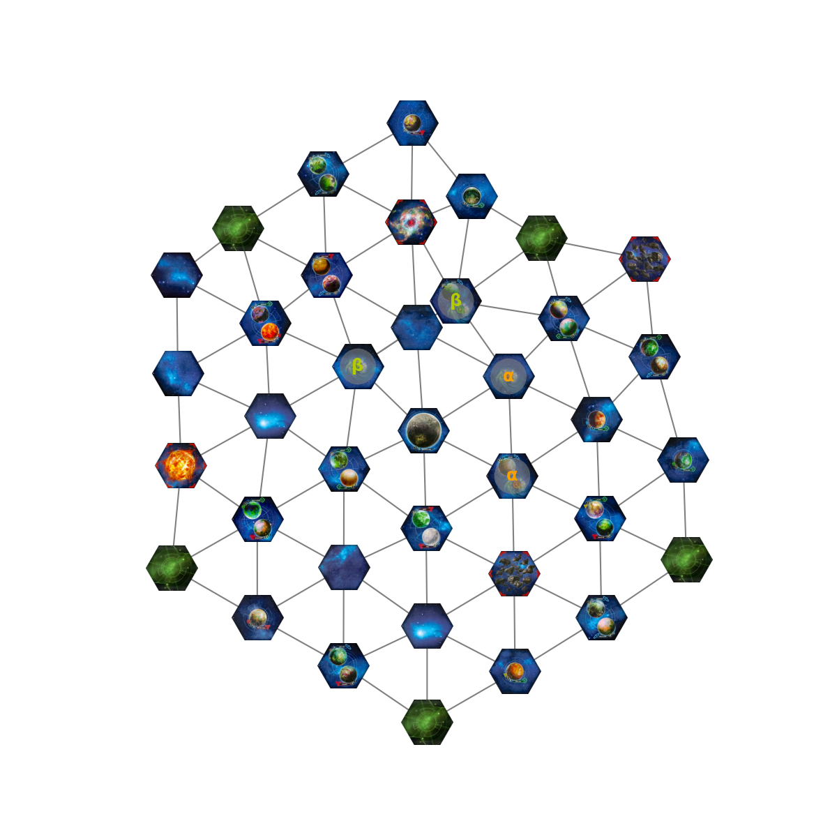
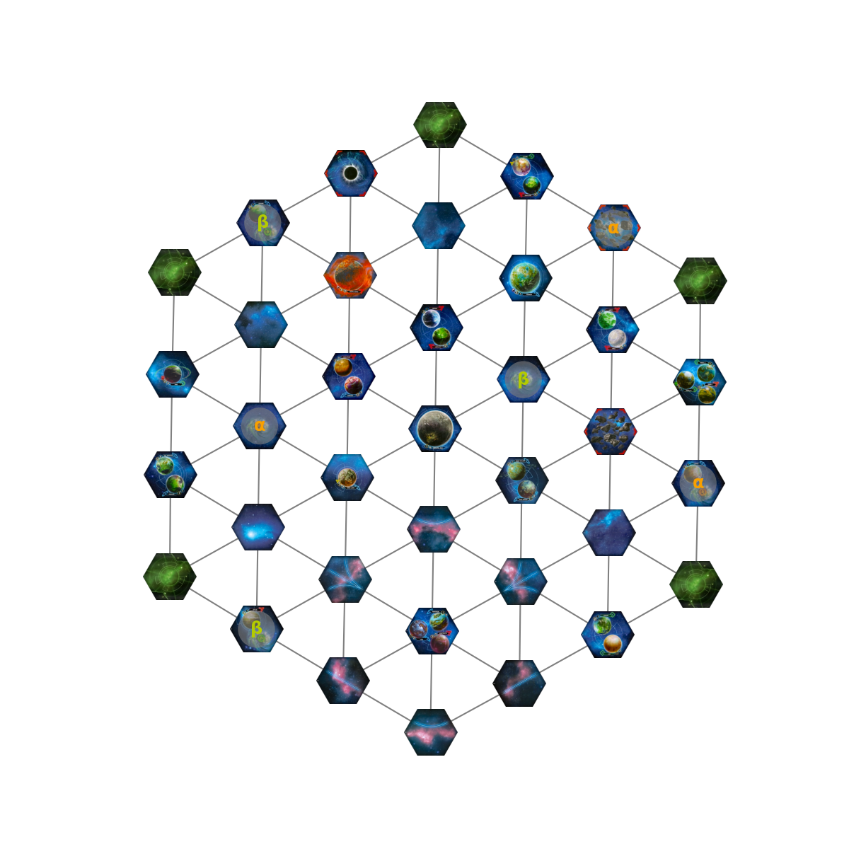
Let’s see what happens if we try to embed a TI map. In TI, tiles are adjacent if their edges are touching, or if they are wormholes with the same letter. In the map below, there are two pairs of worm holes: alpha (orange) and beta (green). You can see that in the embedding, the two beta wormholes are pulled together. The alpha wormholes are unaffected, since they are already adjacent.

What about a more interesting maps? Here is one I played on recently

The whispy lines at the bottom aren’t real tiles, they indicate connections between tiles and are used to balance a five player map. So really, the map looks like this:

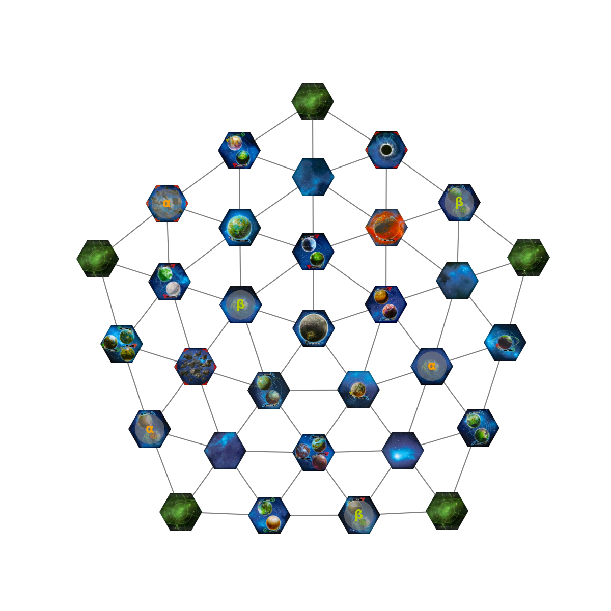
What happens if we add in the wormhole connections?

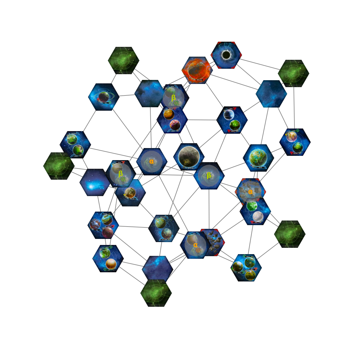
We get an accurate representation of my mental state during that game. Not very useful, how about 3d?

Much better.

How new wormholes change the geometry

Now, TI being TI, the connectivity of the board sometimes changes mid-game (when new wormholes are discovered or when laws are passed which affect movement through wormholes). We can simulate the connectivity changes by slightly modifying the embedding procedure. At step 2., instead of picking the points $P$ randomly, we can use an existing embedding. We then run the optimization step by step, and observe how the optimizer tries to fit the new objective.

Here’s the state after the discovery of the Malice planet, which is connected to a tile via gamma wormhole. I draw Malice as the letter μ.

Since Malice is only connected to one other tile, it is pushed away from everything else, hovering “above” the γ wormhole.

When Malice is activated in the game, it turns into a universal alpha/beta/gamma wormhole. Here is how the board geometry changes as a result:

We can see that it travels into the centre of the representation, in between all the wormholes. The remaining board geometry remains mostly unchanged, aside from γ traveling closer into the centre.

And finally, just for fun, here is the transition between a five player map without wormholes into a map with wormholes.

Actual Applications

Graph planarisation has applications outside of interstellar combat. I learned about it while reading about nonlinear dimensionality reduction. MDS is one of the components of Isomap.

Implementation notes

I have published the code I used to generate the figures and animations here.

The graph embeddings were fit with a few lines of pytorch. I’ll include them here, because using it for simple numeric optimization, outside of the training/inference paradigm, is a trick I only learned recently.

@dataclass(frozen=True)
class Planariser:
    graph: Graph
    num_dims: int
    loss_order: float = 2.0
    seed: int | None = None

    def _init_params(self):
        if self.seed is not None:
            torch.manual_seed(self.seed)
        points = torch.nn.parameter.Parameter(
            torch.Tensor(self.num_dims, self.graph.num_nodes)
        )
        torch.nn.init.normal_(points)
        return points

    def _step(
        self,
        points,
        graph_distances,
        optimizer,
    ) -> float:
        deltas = points.unsqueeze(1) - points.unsqueeze(2)
        euclidian_distances = (
            (deltas ** self.loss_order).abs().sum(axis=0) + EPS
        ) ** (1 / self.loss_order)

        c = 1

        loss = (
            ((euclidian_distances - graph_distances).abs() ** 2)
            / (c + EPS)
        ).sum()

        optimizer.zero_grad()
        loss.backward()
        optimizer.step()
        return loss

    def _get_optimizer(
        self,
        points,
    ):
        return torch.optim.SGD([points])

    def fit_embeddding(
        self,
        num_iterations: int = 1000,
    ) -> npt.NDArray:
        points = self._init_params()
        graph_distances = torch.Tensor(self.graph.pairwise_distances())
        optimizer = self._get_optimizer(points)

        pbar = tqdm(list(range(num_iterations)))
        for iteration in pbar:
            loss = self._step(
                points,
                graph_distances,
                optimizer,
            )
            pbar.set_description(f"Loss: {loss:.2e}")

        return points.detach()

The visualisations were created with matplotlib. For some of the animations, I’ve set the learning rate (lr) parameter of SDG to be much smaller than the default so that the animations come out smoother. I got the TI map tiles from here.

The map we used was made by @MarkusDaBrave.

If you would like to see your own TI map in this representation and run into trouble with the code base, shoot me an email. The next stage of this project is to get AlphaFold to accept TI maps as inputs /s.

---

1. See the original paper here. Their abstract says that they describe “methods to ‘unfold’ and flatten the curved, convoluted surfaces of the brain” but I don’t think any brains were flattened in the making of those maths. ↩

2. Why the square root? Originally a bug, but it helps everything fit quicker and stops larger graphs from overrunning. ↩

3. The original paper simply uses the Newton-Raphson method, I settled for SGD. ↩

4. This reminds me of Levinthal’s paradox and protein folding in general. ↩